Beerbot

Beerbot (Beer Extraction Experimental Robot) is a small mobile robot that finds a can, grabs it and brings it back to where it started, avoiding the obstacles on its way. I built it in 2015 with David Estévez and Enrique Fernández, as the project for the Mobile Robots course of my master’s in robotics at Universidad Carlos III de Madrid.

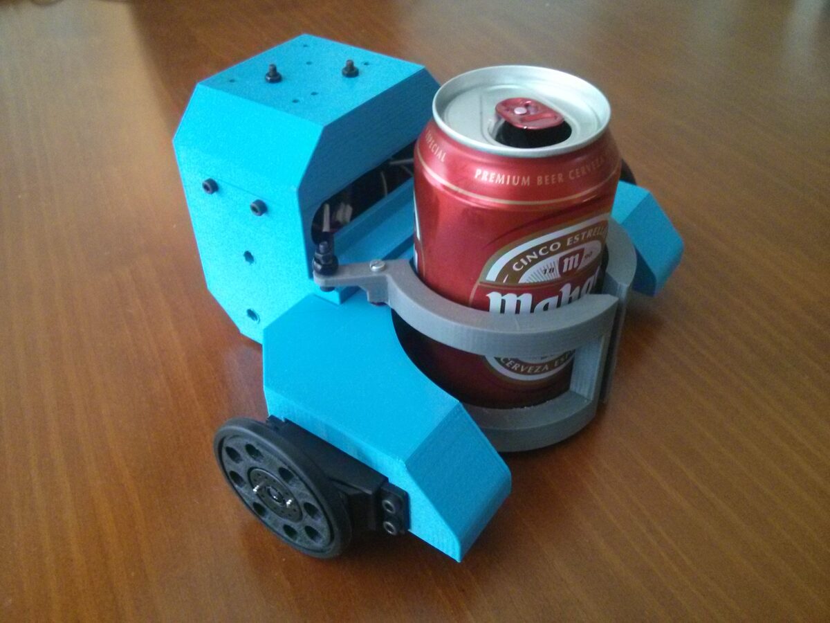
The robot itself has no sensors at all. A camera hanging above the arena sees everything, a computer finds the obstacles, the robot and the can in the image, plans a path and sends wheel speeds to the robot over Bluetooth.

The robot

We designed it in FreeCAD with three requirements in mind: differential drive, a gripper for cans, and parts small enough for a desktop 3D printer.

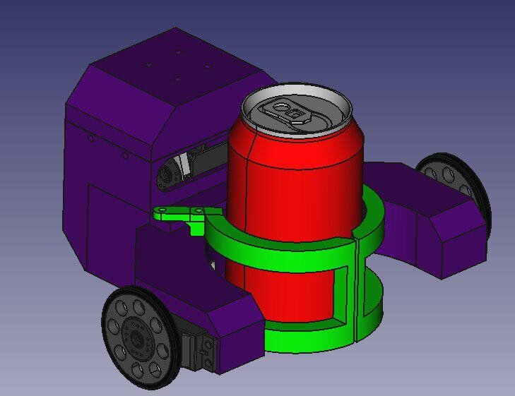
There are eight printed parts, none bigger than 20x20 cm, printed on a BQ Witbox. It has two wheels on the sides and a marble as the third support point.

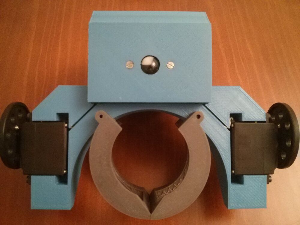
The gripper is moved by a servo through a linkage with ball joints, which is quite robust and lets us set exactly how far it opens. Since it only has to grab cans, it has a small lip at the bottom that lifts the can a bit when it closes, so the can doesn’t drag on the floor.

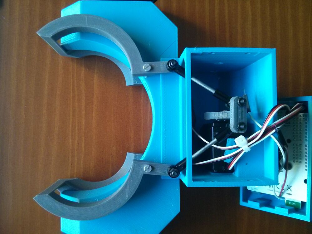
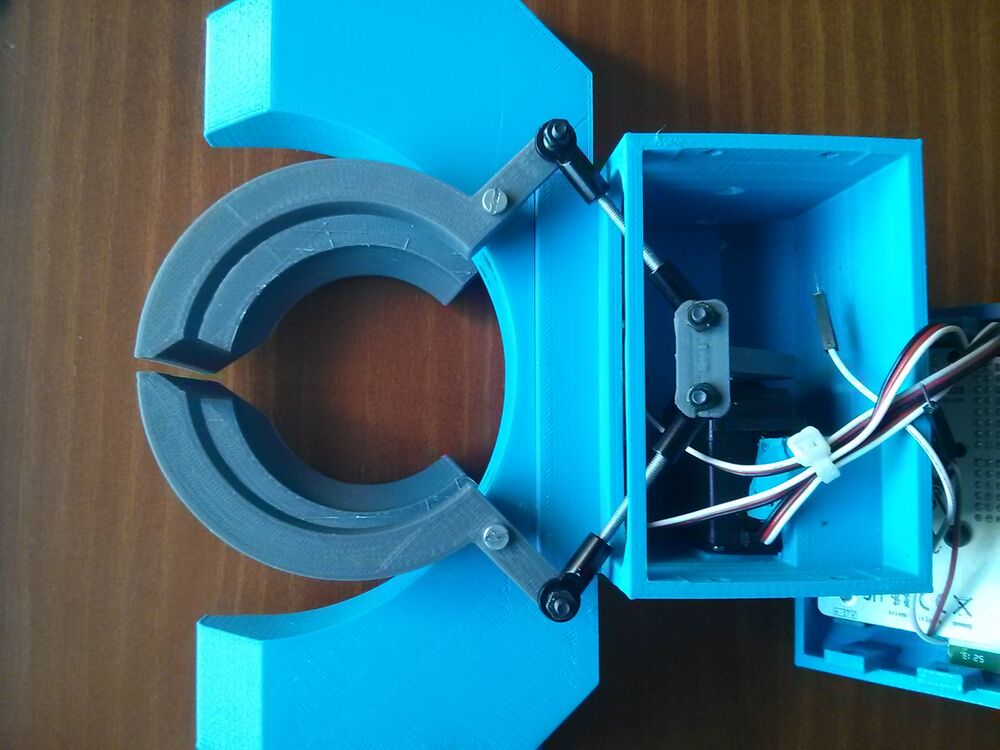
The electronics are as simple as possible: a BQ ZUM board (an Arduino-compatible ATmega328 with Bluetooth built in), two Futaba S3003 servos modified for continuous rotation as the wheel motors, a third, unmodified servo for the gripper and a 2S 1000 mAh LiPo. That’s enough for about an hour of driving, and each test took less than five minutes.

Hacked servos are cheap and easy to find, but they have no real speed control. With the potentiometer disconnected, the servo always thinks it’s at the same position, so the further the commanded position is from it, the faster it spins. We found a range of pulse widths where the speed is roughly linear, and mapped it to one byte per wheel, from -128 to 127, with 0 meaning stopped. Those two bytes are all the computer sends to the robot.

The arena

We used a 2x2 m CEABOT field (the humanoid robot competition), which has a green floor that makes segmentation much easier. The obstacles were whatever we had around the lab, and the camera hung from a cable between two wooden poles.

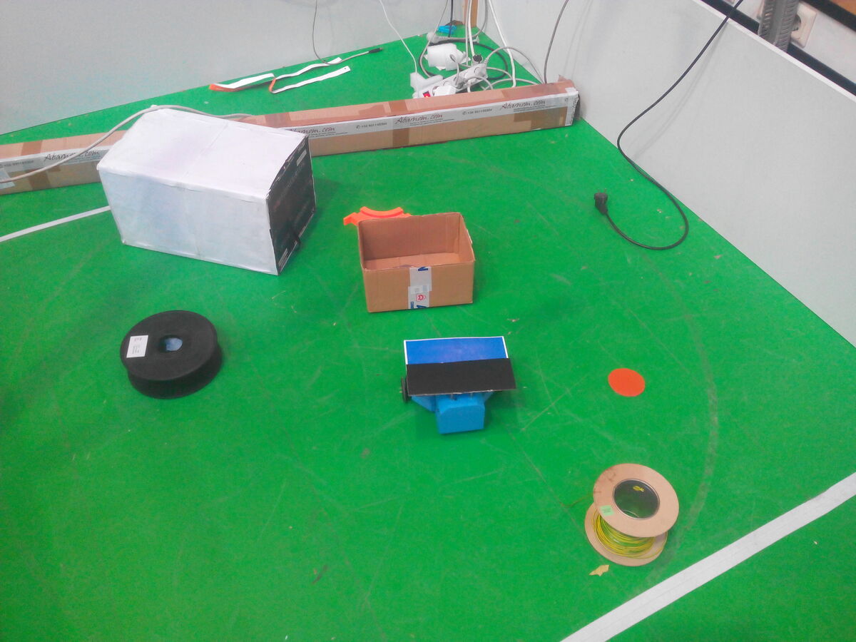
That setup had two problems. The cable made the camera shake, and the lab had big skylights, so the lighting changed all day long, with shadows in some areas and reflections in others. Most of the work ended up being about that.

Vision

First, the camera is calibrated with the OpenCV chessboard pattern to remove the lens distortion. Then each frame goes through these steps:

• Obstacles: everything that isn’t green. The image is thresholded in HSV, cleaned with a 5x5 opening, and the remaining blobs are filtered by size. The result is a binary map for the planner.
• Robot: it carries a marker on top, a rectangle half blue and half black. The black part was a pain with the changing light, so in the end the robot is simply the obstacle that has a blue rectangle inside. Its position is the center of that blob, and its orientation is the vector from that center to the center of the blue part.
• Can: among the obstacles, the ones that are round and the right size. A blob is round when its area is close to the area of the smallest circle that contains it. The colour of the can doesn’t matter.

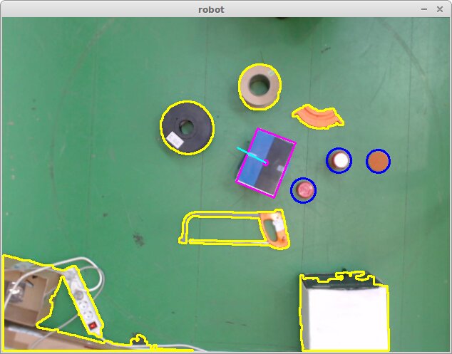
Yellow contours are obstacles, blue circles are the cans and the magenta rectangle is the robot, with its orientation in cyan.

Path planning

For the planning we used Platano, a path planning library we had written for the Task and Motion Planning course of the same master’s. The planner is a quasi-random probabilistic roadmap (Q-PRM): it fills the free space with points, connects the ones that are close to each other, and then searches the resulting graph with A* or Dijkstra.

The difference with a normal PRM is that the points aren’t random. Quasi-random sequences like Halton or Hammersley cover the space more evenly, so you need fewer points to reach narrow passages between obstacles. These are random, Halton and Hammersley points on a real map of the arena:

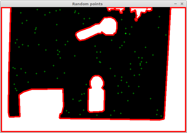
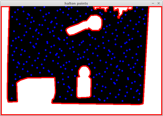
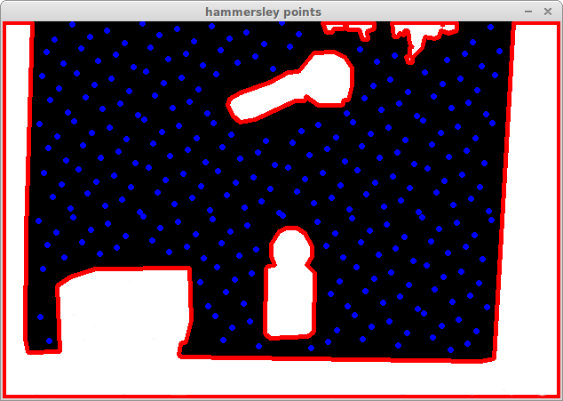
We chose Hammersley, since it gave us a better connected roadmap.

To check collisions quickly, the map is first convolved with a circle the size of the robot, which grows all the obstacles. After that the robot can be treated as a single point: a node is valid if its pixel is free, and an edge is valid if all the points along it are free.

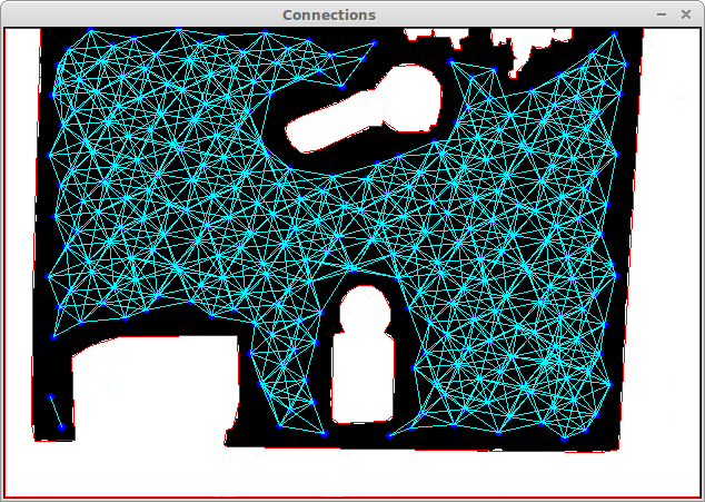
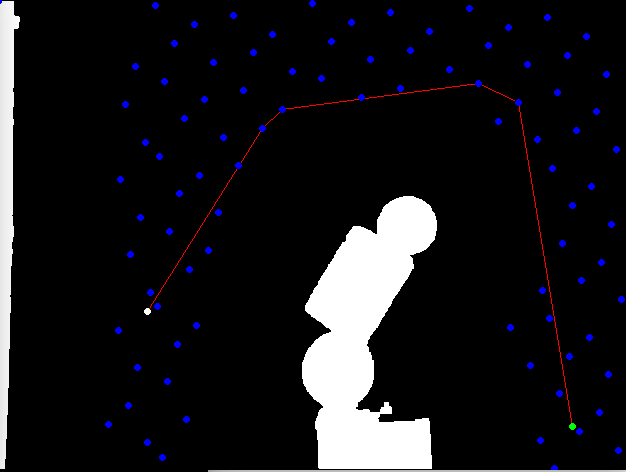
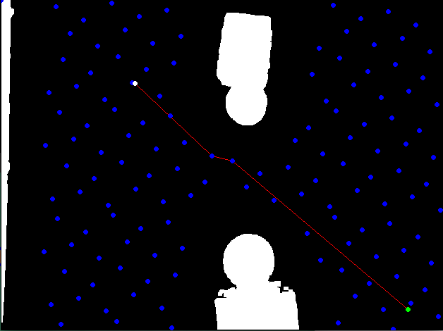
The shortest path through the roadmap is a list of points, and that’s what the robot has to follow:

Control

The control is very simple: turn in place until the robot faces the next point, drive straight to it, and repeat. The camera gives the position and orientation of the robot at every frame, so both moves are closed loop. Once it reaches the can, it closes the gripper and drives the same path back to the start, since the obstacles don’t move and the path is still valid.

Results

We tried three different obstacle layouts and the robot got the can and brought it back in all of them. Here’s the video:

It wasn’t perfect, though:

• When the lighting made the orientation noisy, the robot kept turning back and forth and never moved forward. Tuning the segmentation fixed most of it.
• If it went faster and skipped a point of the path, it turned around to go back to it. It still arrived, it just took longer.
• If the path got too close to the edge of the image and the robot drifted out of view, it lost its position and spun in place until someone put it back.

Things I’d add today: a Kalman filter on the position and orientation, driving and steering at the same time instead of stopping to turn, and replanning on the fly to handle obstacles that move.

Links

• Beerbot repository: FreeCAD and STL files, code and the project report (in Spanish)
• Platano: the path planning library

License

GPLv2